Package com.openinventor.imageviz.engines.edgedetection.edgemarking

Introduction to Edge Marking

See: Description

Class Summary

Class	Description
SoCannyEdgeProcessing	SoCannyEdgeProcessing This engine models the Canny edge detection workflow which is composed of the following steps: 1) Gaussian filtering 2) Gradient computation 3) Non maximum suppression in the gradient direction
SoCannyEdgeProcessing.SbCannyEdgeDetectionDetail	Results details of canny edge detection workflow.
SoDijkstraShortestPathProcessing2d	SoDijkstraShortestPathProcessing2d engine The SoDijkstraShortestPathProcessing2d engine finds the shortest path through an image using local maxima or minima.
SoGradientLocalMaximaProcessing2d	SoGradientLocalMaximaProcessing2d engine The SoGradientLocalMaximaProcessing2d engine suppresses the non-local maxima of the gradient amplitude.
SoGradientLocalMaximaProcessing3d	SoGradientLocalMaximaProcessing3d engine The SoGradientLocalMaximaProcessing3d engine suppresses the non-local maxima of the gradient amplitude.
SoRidgeDetectionProcessing	SoRidgeDetectionProcessing engine The SoRidgeDetectionProcessing engine provides the local maxima of an image.
SoZeroCrossingsProcessing2d	SoZeroCrossingsProcessing2d engine For an introduction to edge marking, see section Introduction to Edge Marking.

Enum Summary

Enum	Description
SoDijkstraShortestPathProcessing2d.AxisSelections
SoDijkstraShortestPathProcessing2d.IntensityModes

Package com.openinventor.imageviz.engines.edgedetection.edgemarking Description

Introduction to Edge Marking

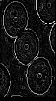
With gradient (ex: SoGradientOperatorProcessing2d) or laplacian (ex: SoRecursiveLaplacianProcessing) engines, a 1D edge was defined as the local maximum of the magnitude of the first derivative, or the zero crossing of the second derivative. Unfortunately, this definition cannot be extended to 2D functions (like for instance SoGradientLocalMaximaProcessing2d). In fact, an edge appears like a crest line on the magnitude of the gradient image and this leads us to define an edge as all the points whose gradient magnitude is maximum along the direction of the gradient, i.e the direction across the edge. This method, referred to as non-maxima suppression, provides thin lines which are much more convenient to handle.

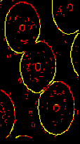
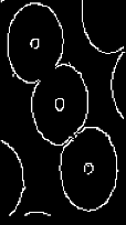
Note that images of zero crossings of the Laplacian result in closed thin lines as they correspond to boundaries between positive and negative regions. Finally, we can take into account the specific geometry of a contour - its pixels are connected by using a more sophisticated threshold, the threshold by hysteresis (SoHysteresisThresholdingProcessing).

This is in fact an intuitive method. We choose a high and low threshold, and , and decide that all the pixels with intensity higher than are edges and those with are edges and those with intensity less than are noise. For the transition area , i.e. pixels with intensity lies between and , we only retain the pixels connected by a line included in to a pixel with a high intensity.